| Introduction | Functions | Data Structures | Demos | FAQ |
GLFM: General Latent Feature Modeling toolbox for python, matlab and R
This code implements a package for General Laten Feature Model (GLFM) suitable for heterogeneous observations. The core code is in C++ and the package provides user interfaces in Python, Matlab and R. Moreover, several demos are provided to illustrate different applications, including missing data estimation and data exploratory analysis, of the GLFM.
To cite this work, please use
 I. Valera, M. F. Pradier, M. Lomeli and Z. Ghahramani,
 "General Latent Feature Model for Heterogeneous Datasets", 2017.
 Available on ArXiv: https://arxiv.org/abs/1706.03779.
GLFM Description
GLFM is a general Bayesian nonparametric latent feature model suitable for heterogeneous datasets, where the attributes describing each object can be either discrete, continuous or mixed variables. Specifically, it accounts for the following types of data:
• Continuous variables:
1. Real-valued, i.e., the attribute takes values in the real line.

2. Positive real-valued, i.e., the attribute takes values in the real line.
• Discrete variables:
1. Categorical data, i.e., the attribute takes a value in a finite unordered set, e.g., {‘blue’,‘red’, ‘black’}.

2. Ordinal data, i.e., the attribute takes values in a finite ordered set, e.g., {‘never’, ‘often’, ‘always’}.

3. Count data, i.e., the attribute takes values in the set {0,...,∞}.
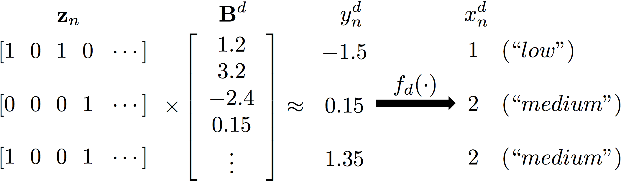
The GLFM builds on the Indian Buffet Process (Griffiths and Ghahramani, 2011), and therefore, it assumes that each observation x_n^d can be explained by a potentially infinite-length binary vector z_n whose elements indicate whether a latent feature is active or not for the n-th object; and a (real-valued) weighting vector B^d, whose elements weight the influence of each latent feature in the d-th attribute. Since the product of the latent feature vector and the weighting vector leads to a real-valued variable, it is necessary to map this variable to the desirable output (continuous or discrete) space, for example, the positive real line. Thus, the GLFM assumes the existence of intermediate Gaussian variables y_n^d, with mean z_nB^d and called pseudo-observation, and a transformation function f_d() that maps this variable into the actual observation x_n^d. As an example, an ordinal attribute taking values in the ordered set {low, medium, high} can be represented using the GLFM as:
For more details on the GLMF, please refer to the research paper.
GLFM Toolbox
You can use GLFM from within Python, Matlab and R. Below we show an example of how to call GLFM for matrix completion and data exploration of a given dataset.
Calling from Python
import GLFM
(hidden) = GLFM.infer(data)
where data is a structure containing:
X: NxD observation matrix of N samples and D dimensions
C: 1xD string array indicating type of data for each dimension
— Alternative calls —
import GLFM
hidden = GLFM.infer(data, hidden);
OR
import GLFM
hidden = GLFM.infer(data, hidden, params);
where hidden is a structure of latent variables:
Z: NxK binary matrix of feature assignments (initialization for the IBP)
and params is a structure containing all simulation parameters and model hyperparameters (see Data Structures for further details).
Calling from Matlab
hidden = GLFM_infer(data);
where data is a structure containing:
X: NxD observation matrix of N samples and D dimensions
C: 1xD string array indicating type of data for each dimension
— Alternative calls —
hidden = GLFM_infer(data, hidden);
OR
hidden = GLFM_infer(data, hidden, params);
where hidden is a structure of latent variables:
Z: NxK binary matrix of feature assignments (initialization for the IBP)
and params is a structure containing all simulation parameters and model hyperparameters (see Data Structures for further details).
Calling from R
output <- GLFM_infer(data)
where data is a structure containing:
X: NxD observation matrix of N samples and D dimensions
C: 1xD string array indicating type of data for each dimension
and output is a list containing the lists hidden and params.
— Alternative calls —
output <- GLFM_infer(data,hidden)
OR
output = GLFM_infer(data, list(hidden, params));
where hidden is a list of latent variables:
Z: NxK binary matrix of feature assignments (initialization for the IBP)
and params is a list containing all simulation parameters and model hyperparameters (see Data Structures for further details). The output list contains the output lists hidden and params.
Requirements
The main requirements include a gcc compiler suitable for your OS and the GNU GSLlibrary.
• For Python:
- Python 2.7
- Anaconda (install at https://www.anaconda.com/download/)
- gcc compiler and qt functionality (these modules are normally already available)
  If not, it can be installed in Ubuntu as:

        sudo apt-get install build-essential
        sudo apt-get install python-qt4
• For Matlab:
- Matlab 2012b or higher
- GNU GSLlibrary
    In UBUNTU: sudo apt-get install libgsl0ldbl or sudo apt-get install libgsl0-dev
- GMP library
    In UBUNTU: sudo apt-get install libgmp3-dev
• For R:
- R or Rstudio
- GNU GSL library (e.g. libgsl0-dev on Debian or Ubuntu)
- Rcpp for seamless R and C++ integration
Compilation Instructions
In order to run GLFM on your data, you need to:
1) Download the latest git repository (command: “git clone https://github.com/ivaleraM/GLFM.git”)
2) Compile the C++ code as
**For PYTHON** (in a terminal):
    - Go to folder "GLFM/install/"
    - Run command: >> bash install_for_python.sh

**For MATLAB** (in Matlab workspace):
    - Add path "GLFM/src/Ccode" and its children directories to Matlab workspace
    - From matlab command window, execute: >> mex  -lgsl -lgmp -lgslcblas IBPsampler.cpp

**For R** (in a terminal):
    - Go to folder "GLFM/install/"
    - Run command: >> bash install_for_R.sh
3) Check the success of the compilation by running the scipt ‘demo_GLFM_test’ available for Python, Matlab and R in the ‘demos’ folder.
GLFM Demos
The folder ‘‘demos’’ contain scripts, as well as Jupiter notebooks, with application examples of the GLFM, including missing data estimation (a.k.a. matrix completion) and data exploratory analysis. As an example, the script `demo_toyImages’ replicates the example of the IBP linear-Gaussian model in (Griffiths and Ghahramani, 2011) by generating a small set of images composed by different combinations of four original images plus additive Gaussian noise. Using the GLFM, we are able to recover the original images seamlessly. Other examples include demo_matrix_completion_MNIST, demo_data_exploration_counties, and demo_data_exploration_prostate, available for PYTHON, Matlab and R. For more detail, please visit our demo website.
Licence
The Python and Matlab implementations are under MIT license. The R implementation extends the RcppGSLExample, and therefore, is under GPL (>= 2) license.
Contact
For further information or contact:
Isabel Valera: isabel.valera.martinez (at) gmail.com
Melanie F. Pradier: melanie.fpradier (at) gmail.com
Maria Lomeli: maria.lomeli  (at) eng.cam.ac.uk